机器学习实战

化妆学校实习机会：提升实战经验的好途径 #生活技巧# #化妆打扮技巧# #化妆学校#

import pandas as pd df = pd.read_csv('F:/MNIST/mnist.csv', header=None) df.head() 123 0123456789...77577677777877978078178278378405000000000...000000000010000000000...000000000024000000000...000000000031000000000...000000000049000000000...0000000000

5 rows × 785 columns

import numpy as np df = df.reindex(np.random.permutation(df.index)) # 打乱顺序的方法 x = df.drop(0, axis=1) y = df[0] print('X的概况：', x.shape) print('Y的概况：', y.shape) x_train, x_test, y_train, y_test = x[:60000], x[60000:], y[:60000], y[60000:] 12345678

X的概况： (70000, 784) Y的概况： (70000,) 12

""" data.irow(0) #取data的第一行 data.icol(0) #取data的第一列 data.ix[1:2] #返回第2行的第三种方法，返回的是DataFrame，跟data[1:2]同 data[1:2] #返回第2行，从0计，返回的是单行，通过有前后值的索引形式， #如果采用data[1]则报错 """ print(y[36000]) %matplotlib inline import matplotlib import matplotlib.pyplot as plt some_digit = x.loc[[36000]].values some_digit_image = some_digit.reshape(28, 28) plt.imshow(some_digit_image, cmap=matplotlib.cm.binary, interpolation='nearest') plt.axis('off') plt.show()

123456789101112131415161718

9 1

print(y_train.head()) y_test 12

41266 1 719 5 69105 0 58965 1 61484 1 Name: 0, dtype: int64 18193 9 8664 1 24326 3 59176 1 28477 5 40056 1 44939 5 32688 3 30398 3 1460 4 64379 4 66269 7 26930 0 33416 1 5443 1 61529 4 54202 5 64308 1 51409 7 10533 7 10417 2 54426 7 55812 4 65474 4 51762 5 8364 7 8601 9 69603 2 1043 7 28068 2 .. 48235 4 30295 6 20432 2 12970 7 9458 0 65275 5 8466 4 62936 4 21244 5 3176 2 34733 4 2974 0 66701 0 12519 5 46747 1 34662 0 50322 5 39379 6 33823 0 60482 7 48927 9 7176 1 49476 5 33086 1 58856 8 1062 5 63524 6 65577 4 26155 9 55798 6 Name: 0, Length: 10000, dtype: int64

12345678910111213141516171819202122232425262728293031323334353637383940414243444546474849505152535455565758596061626364656667686970717273

y_train_9 = (y_train==9) y_test_9 = (y_test==9) #print(y_test[[2797]]) #y_test_9 123456

# 使用随机梯度下降（SGD）训练模型 from sklearn.linear_model import SGDClassifier sgd_clf = SGDClassifier(random_state=42) sgd_clf.fit(x_train, y_train_9) 123456

SGDClassifier(alpha=0.0001, average=False, class_weight=None, early_stopping=False, epsilon=0.1, eta0=0.0, fit_intercept=True, l1_ratio=0.15, learning_rate='optimal', loss='hinge', max_iter=1000, n_iter_no_change=5, n_jobs=None, penalty='l2', power_t=0.5, random_state=42, shuffle=True, tol=0.001, validation_fraction=0.1, verbose=0, warm_start=False) 123456

sgd_clf.predict(x.loc[[30069,42882,167,33531,11688,26571,16734,14324]]) # sgd_clf.predict([some_digit]) # 这种语法错误为：Found array with dim 3. Estimator expected <= 2. 123

array([ True, True, True, True, True, True, True, True]) 1

# 使用cross_val_score模块的3折交叉验证方法改进SGD模型 from sklearn.model_selection import cross_val_score # 采用K-fold交叉验证发，3个折叠 cross_val_score(sgd_clf, x_train, y_train_9, cv=3, scoring='accuracy') 123

array([0.92680366, 0.9418 , 0.9439472 ]) 1

# 使用混淆矩阵（cross_val_predict）方法获取预测的真OR假结果，以便计算精确率和召回率 from sklearn.model_selection import cross_val_predict # 先返回每个折叠的预测，每个预测都是在训练期间从未见过的 y_train_pred = cross_val_predict(sgd_clf, x_train, y_train_9, cv=3) 123

y_train_pred 1

array([False, False, False, ..., False, False, False]) 1

# 使用生成的y_train_pred（预测结果正确与否的列表）与真实值计算精确率和召回率 # 手工算法 from sklearn.metrics import confusion_matrix print(confusion_matrix(y_train_9, y_train_pred)) """ 真负类TN 假正类FP 假负类FN 真正类TP """ jingdu = 3637 / (3637+2281) zhaohuilv = 3637 / (3637+1468) print('精度：', jingdu) print('召回率：', zhaohuilv) 123456789101112

[[52614 1468] [ 2281 3637]] 精度： 0.6145657316661034 召回率： 0.7124387855044074 1234

# 使用sklearn.metrics中的precision_score和recall_score自动计算精确率和召回率 from sklearn.metrics import precision_score,recall_score precision_score(y_train_9, y_train_pred) 1234

0.7124387855044074 1

recall_score(y_train_9, y_train_pred) 1

0.6145657316661034 1

# 使用sklearn.metrics中的f1_score模块，自动计算F1分数（2*精度*召回率 / (精度 + 召回率)） from sklearn.metrics import f1_score f1_score(y_train_9, y_train_pred) 123

0.6598929511022407 1

# 设定阈值来改变精度和召回率，主意参数：method='decision_function' # method='decision_function'这个参数返回的是计算得出的分数。可以用来设定阈值 #from sklearn.model_selection import cross_val_predict # 先返回每个折叠的预测，每个预测都是在训练期间从未见过的 #y_train_pred = cross_val_predict(sgd_clf, x_train, y_train_9, cv=3) y_scores = cross_val_predict(sgd_clf, x_train, y_train_9, method='decision_function') y_scores 12345678

D:\Anaconda3\lib\site-packages\sklearn\model_selection\_split.py:1978: FutureWarning: The default value of cv will change from 3 to 5 in version 0.22. Specify it explicitly to silence this warning. warnings.warn(CV_WARNING, FutureWarning) array([-42620.62981929, -51693.91890067, -39176.69145394, ..., -22254.03321689, -53437.33278592, -33654.56993053]) 123456789

# 画出精确率和召回率的图 from sklearn.metrics import precision_recall_curve precisions, recalls, thresholds = precision_recall_curve(y_train_9, y_scores) def plot_pre_recall_vs_thre(precisions, recalls, thresholds): plt.plot(thresholds, precisions[:-1], 'b--',label='Precision') plt.plot(thresholds, recalls[:-1],'g--', label='recall') plt.xlabel('Threshold') plt.legend(loc='upper left') plt.ylim([0,1]) plot_pre_recall_vs_thre(precisions, recalls, thresholds) plt.show() 12345678910111213

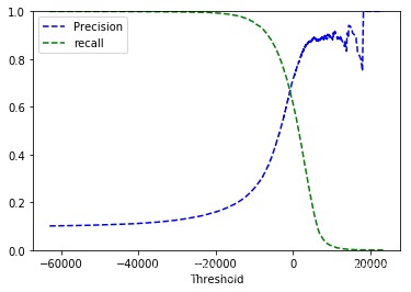
y_train_pred_90 = (y_scores > 10000) precision_score(y_train_9, y_train_pred_90) 12

0.8898305084745762 1

recall_score(y_train_9, y_train_pred_90) 1

0.01774248056775938 1

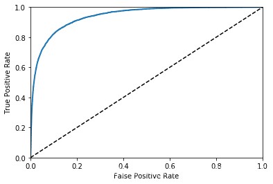
# ROC曲线：特异度和灵敏度的关系 from sklearn.metrics import roc_curve fpr, tpr, thresholds = roc_curve(y_train_9, y_scores) def plot_roc_curve(fpr, tpr, label=None): plt.plot(fpr, tpr, linewidth=2, label=label) plt.plot([0,1], [0,1], 'k--') plt.axis([0,1,0,1]) plt.xlabel('False Positive Rate') plt.ylabel('True Positive Rate') plot_roc_curve(fpr, tpr) plt.show() 1234567891011121314

# 训练一个随机森林，与SGD分类在ROC曲线上进行对比 from sklearn.ensemble import RandomForestClassifier forest_clf = RandomForestClassifier(random_state=42) y_probas_forest = cross_val_predict(forest_clf, x_train, y_train_9, cv=10, method='predict_proba') 12345

D:\Anaconda3\lib\site-packages\sklearn\ensemble\forest.py:245: FutureWarning: The default value of n_estimators will change from 10 in version 0.20 to 100 in 0.22. "10 in version 0.20 to 100 in 0.22.", FutureWarning) D:\Anaconda3\lib\site-packages\sklearn\ensemble\forest.py:245: FutureWarning: The default value of n_estimators will change from 10 in version 0.20 to 100 in 0.22. "10 in version 0.20 to 100 in 0.22.", FutureWarning) D:\Anaconda3\lib\site-packages\sklearn\ensemble\forest.py:245: FutureWarning: The default value of n_estimators will change from 10 in version 0.20 to 100 in 0.22. "10 in version 0.20 to 100 in 0.22.", FutureWarning) D:\Anaconda3\lib\site-packages\sklearn\ensemble\forest.py:245: FutureWarning: The default value of n_estimators will change from 10 in version 0.20 to 100 in 0.22. "10 in version 0.20 to 100 in 0.22.", FutureWarning) D:\Anaconda3\lib\site-packages\sklearn\ensemble\forest.py:245: FutureWarning: The default value of n_estimators will change from 10 in version 0.20 to 100 in 0.22. "10 in version 0.20 to 100 in 0.22.", FutureWarning) D:\Anaconda3\lib\site-packages\sklearn\ensemble\forest.py:245: FutureWarning: The default value of n_estimators will change from 10 in version 0.20 to 100 in 0.22. "10 in version 0.20 to 100 in 0.22.", FutureWarning) D:\Anaconda3\lib\site-packages\sklearn\ensemble\forest.py:245: FutureWarning: The default value of n_estimators will change from 10 in version 0.20 to 100 in 0.22. "10 in version 0.20 to 100 in 0.22.", FutureWarning) D:\Anaconda3\lib\site-packages\sklearn\ensemble\forest.py:245: FutureWarning: The default value of n_estimators will change from 10 in version 0.20 to 100 in 0.22. "10 in version 0.20 to 100 in 0.22.", FutureWarning) D:\Anaconda3\lib\site-packages\sklearn\ensemble\forest.py:245: FutureWarning: The default value of n_estimators will change from 10 in version 0.20 to 100 in 0.22. "10 in version 0.20 to 100 in 0.22.", FutureWarning) D:\Anaconda3\lib\site-packages\sklearn\ensemble\forest.py:245: FutureWarning: The default value of n_estimators will change from 10 in version 0.20 to 100 in 0.22. "10 in version 0.20 to 100 in 0.22.", FutureWarning)

1234567891011121314151617181920

# 随机森林中，使用参数method='predict_proba'，返回的是概率值 y_probas_forest 12

array([[1., 0.], [1., 0.], [1., 0.], ..., [1., 0.], [1., 0.], [1., 0.]]) 1234567

y_scores_forest = y_probas_forest[:, 1] fpr_forest, tpr_forest, thresholds_forest = roc_curve(y_train_9, y_scores_forest) plt.plot(fpr, tpr, 'b', label='SGD') plot_roc_curve(fpr_forest, tpr_forest, 'Random Forest') plt.legend(loc='bottom right') plt.show() 1234567

D:\Anaconda3\lib\site-packages\matplotlib\legend.py:497: UserWarning: Unrecognized location "bottom right". Falling back on "best"; valid locations arebestupper rightupper leftlower leftlower rightrightcenter leftcenter rightlower centerupper centercenter % (loc, '\n\t'.join(self.codes))) 1234567891011121314

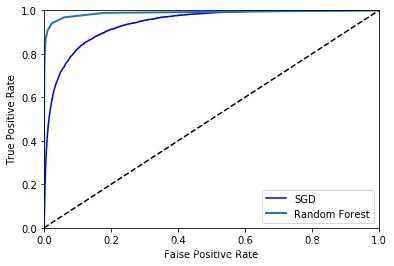
from sklearn.metrics import roc_auc_score print(roc_auc_score(y_train_9, y_scores)) print(roc_auc_score(y_train_9, y_scores_forest)) 1234

0.9401824847125175 0.9883210685077506 12

# 多类别分类器 # OvA——OvO # 先使用SGD对所有标签进行训练试试 sgd_clf.fit(x_train, y_train) 12345

SGDClassifier(alpha=0.0001, average=False, class_weight=None, early_stopping=False, epsilon=0.1, eta0=0.0, fit_intercept=True, l1_ratio=0.15, learning_rate='optimal', loss='hinge', max_iter=1000, n_iter_no_change=5, n_jobs=None, penalty='l2', power_t=0.5, random_state=42, shuffle=True, tol=0.001, validation_fraction=0.1, verbose=0, warm_start=False) 123456

sgd_clf.predict(x.loc[[36000]]) 1

array([4], dtype=int64) 1

# 看看sklearn中二分类器是如何进行多类别分类的，需要看decision_function()分数 # 很明显，分类为9的分数为-2712，是最大的，所以分类为9，结果也是正确的。 some_digit_scores = sgd_clf.decision_function(x.loc[[36000]]) print(some_digit_scores) print(np.argmax(some_digit_scores)) # np.argmax() 求最大的nampy方法 print(sgd_clf.classes_) # 查看原始结果方法 123456

[[-39761.98821912 -22916.54645981 -18184.28472608 1016.42192678 2300.61774756 -6673.18271756 -40432.41849423 -13508.94695046 -2635.88432119 -2399.9387372 ]] 4 [0 1 2 3 4 5 6 7 8 9] 12345

# 使用交叉验证方法评估SGD的准确率 cross_val_score(sgd_clf, x_train, y_train, cv=3, scoring='accuracy') 12

array([0.85907114, 0.87885 , 0.8819823 ]) 1

# 使用多分类器“随机森林”算法再试试看 forest_clf.fit(x_train, y_train) 123

D:\Anaconda3\lib\site-packages\sklearn\ensemble\forest.py:245: FutureWarning: The default value of n_estimators will change from 10 in version 0.20 to 100 in 0.22. "10 in version 0.20 to 100 in 0.22.", FutureWarning) RandomForestClassifier(bootstrap=True, class_weight=None, criterion='gini', max_depth=None, max_features='auto', max_leaf_nodes=None, min_impurity_decrease=0.0, min_impurity_split=None, min_samples_leaf=1, min_samples_split=2, min_weight_fraction_leaf=0.0, n_estimators=10, n_jobs=None, oob_score=False, random_state=42, verbose=0, warm_start=False) 1234567891011121314

# 返回概率值，发现结果是9的概率最大，所以返回结果是9 forest_clf.predict_proba(x.loc[[36000]]) 12

array([[0., 0., 0., 0., 0., 0., 0., 0., 0., 1.]]) 1

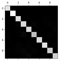
# 错误分析 # 使用cross_val_predict()函数进行预测，然后调用confusion_matrix()函数 y_train_pred_final = cross_val_predict(forest_clf, x_train, y_train, cv=3) conf_mx = confusion_matrix(y_train, y_train_pred_final) conf_mx 12345

array([[5853, 2, 18, 6, 5, 15, 30, 2, 28, 2], [ 1, 6618, 39, 19, 15, 10, 7, 11, 11, 5], [ 54, 20, 5686, 39, 40, 7, 23, 57, 47, 5], [ 36, 21, 147, 5646, 7, 119, 10, 52, 84, 36], [ 18, 13, 34, 10, 5572, 10, 40, 19, 23, 117], [ 50, 21, 31, 206, 35, 4948, 56, 12, 54, 30], [ 57, 15, 26, 6, 31, 69, 5643, 1, 24, 2], [ 13, 28, 96, 27, 82, 4, 2, 5861, 13, 79], [ 29, 47, 104, 133, 61, 106, 44, 29, 5240, 78], [ 33, 20, 31, 85, 193, 41, 6, 89, 65, 5355]], dtype=int64) 1234567891011

plt.matshow(conf_mx, cmap=plt.cm.gray) plt.show() 12

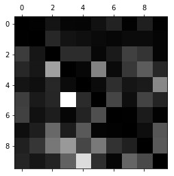
row_sums = conf_mx.sum(axis=1, keepdims=True) norm_conf_mx = conf_mx / row_sums np.fill_diagonal(norm_conf_mx, 0) plt.matshow(norm_conf_mx, cmap=plt.cm.gray) plt.show() 12345

# 多标签分类 # 希望分类器为每个样本产生多个类别（如一张照片里识别出多个人） # 分类器可以输出多个二元标签。 # 这种分类叫做，多标签分类系统 from sklearn.neighbors import KNeighborsClassifier y_train_large = (y_train >= 7) y_train_odd = (y_train % 2 == 1) y_multilabel = np.c_[y_train_large, y_train_odd] knn_clf = KNeighborsClassifier() knn_clf.fit(x_train, y_multilabel) 123456789101112

KNeighborsClassifier(algorithm='auto', leaf_size=30, metric='minkowski', metric_params=None, n_jobs=None, n_neighbors=5, p=2, weights='uniform') 123

knn_clf.predict(x.loc[[36000]]) 1

array([[ True, True]]) 1

# 多标签分类的评估 y_train_knn_pred = cross_val_predict(knn_clf, x_train, y_train, cv=3) f1_score(y_train, y_train_knn_pred, average='macro') 1234

网址：机器学习实战 https://www.yuejiaxmz.com/news/view/1006017

相关内容

机器学习实战指南
《机器学习实战》第六章
机器学习实战之数回归，CART算法
深度学习实战8
深度学习实战98
【机器学习】机器学习：驱动个性化服务行业的新引擎
学机器学习可以做什么？
机器学习提升法
【机器学习PAI实战】—— 玩转人工智能之美食推荐
机器学习优化策略

随便看看