python可视化编程实例(matplotlib)

编程基础：Python入门教程和JavaScript实战案例 #生活技巧# #学习技巧# #技能训练指南#

1 直方图

import matplotlib.pylab as plt

plt.style.use('ggplot')

customers = ['ABC', 'DEF', 'GHI', 'JKL', 'MNO']

customers_index = range(len(customers))

sale_amounts = [127, 90, 201, 111, 232]

fig = plt.figure()

ax1 = fig.add_subplot(1, 1, 1)

ax1.bar(customers_index, sale_amounts, align='center', color='darkblue')

ax1.xaxis.set_ticks_position('bottom')

ax1.yaxis.set_ticks_position('left')

plt.xticks(customers_index, customers, rotation=0, fontsize='small')

plt.xlabel('Customer Name')

plt.ylabel('Sale Amount')

plt.title('Sale Amount per Customer')

plt.savefig('bar_plot.png', dpi=400, bbox_inches='tight')

plt.show()

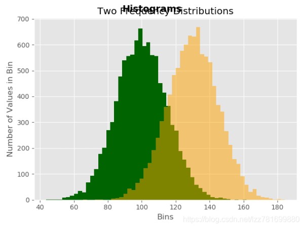
频率分布图

import numpy as np

import matplotlib.pyplot as plt

plt.style.use('ggplot')

mu1, mu2, sigma = 100, 130, 15

x1 = mu1 + sigma*np.random.randn(10000)

x2 = mu2 + sigma*np.random.randn(10000)

fig = plt.figure()

ax1 = fig.add_subplot(1, 1, 1)

n, bins, patches = ax1.hist(x1, bins=50, normed=False, color='darkgreen')

n, bins, patches = ax1.hist(x2, bins=50, normed=False, color='orange', alpha=0.5)

ax1.xaxis.set_ticks_position('bottom')

ax1.yaxis.set_ticks_position('left')

plt.xlabel('Bins')

plt.ylabel('Number of Values in Bin')

fig.suptitle('Histograms', fontsize=14, fontweight='bold')

ax1.set_title('Two Frequency Distributions')

plt.savefig('histogram.png', dpi=400, bbox_inches='tight')

plt.show()

from numpy.random import randn

import matplotlib.pyplot as plt

plt.style.use('ggplot')

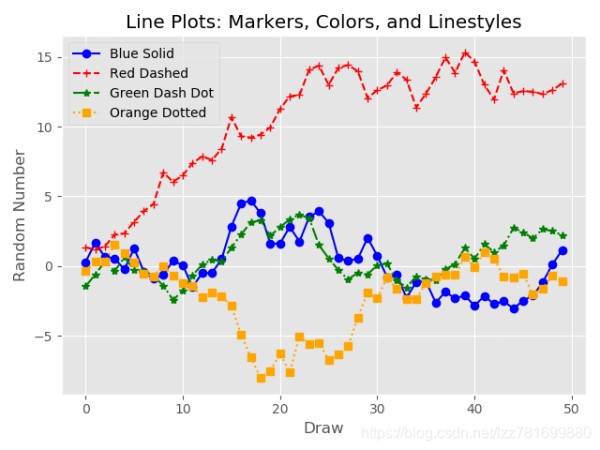
plot_data1 = randn(50).cumsum()

plot_data2 = randn(50).cumsum()

plot_data3 = randn(50).cumsum()

plot_data4 = randn(50).cumsum()

fig = plt.figure()

ax1 = fig.add_subplot(1, 1, 1)

ax1.plot(plot_data1, marker=r'o', color=u'blue', linestyle='-',label='Blue Solid')

ax1.plot(plot_data2, marker=r'+', color=u'red', linestyle='--',label='Red Dashed')

ax1.plot(plot_data3, marker=r'*', color=u'green', linestyle='-.',label='Green Dash Dot')

ax1.plot(plot_data4, marker=r's', color=u'orange', linestyle=':',label='Orange Dotted')

ax1.xaxis.set_ticks_position('bottom')

ax1.yaxis.set_ticks_position('left')

ax1.set_title('Line Plots: Markers, Colors, and Linestyles')

plt.xlabel('Draw')

plt.ylabel('Random Number')

plt.legend(loc='best')

plt.savefig('line_plot.png', dpi=400, bbox_inches='tight')

plt.show()

'

 

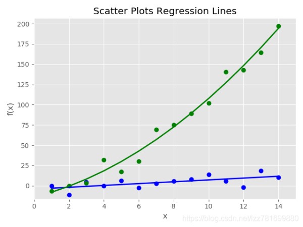
# 散点图

import numpy as np

import matplotlib.pyplot as plt

plt.style.use('ggplot')

x = np.arange(start=1., stop=15., step=1.)

y_linear = x + 5 * np.random.randn(14)

y_quadratic = x**2 + 10 * np.random.randn(14)

fn_linear = np.poly1d(np.polyfit(x, y_linear, deg=1))

fn_quadratic = np.poly1d(np.polyfit(x, y_quadratic, deg=2))

fig = plt.figure()

ax1 = fig.add_subplot(1,1,1)

ax1.plot(x, y_linear, 'bo', x, y_quadratic, 'go',x, fn_linear(x), 'b-', x, fn_quadratic(x), 'g-', linewidth=2.)

ax1.xaxis.set_ticks_position('bottom')

ax1.yaxis.set_ticks_position('left')

ax1.set_title('Scatter Plots Regression Lines')

plt.xlabel('x')

plt.ylabel('f(x)')

plt.xlim((min(x)-1., max(x)+1.))

plt.ylim((min(y_quadratic)-10., max(y_quadratic)+10.))

plt.savefig('scatter_plot.png', dpi=400, bbox_inches='tight')

plt.show()

 

# 箱线图

import numpy as np

import matplotlib.pyplot as plt

plt.style.use('ggplot')

N = 500

normal = np.random.normal(loc=0.0, scale=1.0, size=N)

lognormal = np.random.lognormal(mean=0.0, sigma=1.0, size=N)

index_value = np.random.random_integers(low=0, high=N-1, size=N)

normal_sample = normal[index_value]

lognormal_sample = lognormal[index_value]

box_plot_data = [normal,normal_sample,lognormal,lognormal_sample]

fig = plt.figure()

ax1 = fig.add_subplot(1,1,1)

box_labels = ['normal','normal_sample','lognormal','lognormal_sample']

ax1.boxplot(box_plot_data, notch=False, sym='.', vert=True, whis=1.5,showmeans=True, labels=box_labels)

ax1.xaxis.set_ticks_position('bottom')

ax1.yaxis.set_ticks_position('left')

ax1.set_title('Box Plots: Resampling of Two Distributions')

ax1.set_xlabel('Distribution')

ax1.set_ylabel('Value')

plt.savefig('box_plot.png', dpi=400, bbox_inches='tight')

plt.show()

 

网址：python可视化编程实例(matplotlib) https://www.yuejiaxmz.com/news/view/518049

相关内容

Python中的Numpy、SciPy、MatPlotLib安装与配置
Python制作生活工具
Python在智能家居自动化中的实战应用：Home Assistant集成与扩展
用matplotlib绘制饼图（学习规划——时间馅饼）
【Python】实现一个个人理财助手小程序
Python数据可视化
掌握这17个Python自动化操作，简化你的日常工作流程，提升工作效率！
Python中的生活数据分析与个人健康监测.pptx
学了python究竟有什么用，实际应用场景有哪些？我整理了8个应用领域
Python编程：美好生活的秘密武器

随便看看