李弘毅机器学习笔记：回归演示

学习机器学习基础知识，如线性回归 #生活技巧# #工作学习技巧# #数字技能学习#

李弘毅机器学习笔记：回归演示

现在假设有10个x_data和y_data，x和y之间的关系是y_data=b+w*x_data。b，w都是参数，是需要学习出来的。现在我们来练习用梯度下降找到b和w。

x_data = [338., 333., 328., 207., 226., 25., 179., 60., 208., 606.] y_data = [640., 633., 619., 393., 428., 27., 193., 66., 226., 1591.] x_d = np.asarray(x_data) y_d = np.asarray(y_data) 1234

先给b和w一个初始值，计算出b和w的偏微分

# linear regression b = -120 w = -4 lr = 0.0000001 iteration = 100000 b_history = [b] w_history = [w] import time start = time.time() for i in range(iteration): b_grad=0.0 w_grad=0.0 for n in range(len(x_data)) b_grad=b_grad-2.0*(y_data[n]-n-w*x_data[n])*1.0 w_grad= w_grad-2.0*(y_data[n]-n-w*x_data[n])*x_data[n] # update param b -= lr * b_grad w -= lr * w_grad b_history.append(b) w_history.append(w)

12345678910111213141516171819202122232425

# plot the figure plt.subplot(1, 2, 1) C = plt.contourf(x, y, Z, 50, alpha=0.5, cmap=plt.get_cmap('jet')) # 填充等高线 # plt.clabel(C, inline=True, fontsize=5) plt.plot([-188.4], [2.67], 'x', ms=12, mew=3, color="orange") plt.plot(b_history, w_history, 'o-', ms=3, lw=1.5, color='black') plt.xlim(-200, -100) plt.ylim(-5, 5) plt.xlabel(r'$b$') plt.ylabel(r'$w$') plt.title("线性回归") plt.subplot(1, 2, 2) loss = np.asarray(loss_history[2:iteration]) plt.plot(np.arange(2, iteration), loss) plt.title("损失") plt.xlabel('step') plt.ylabel('loss') plt.show()

1234567891011121314151617181920

输出结果如图

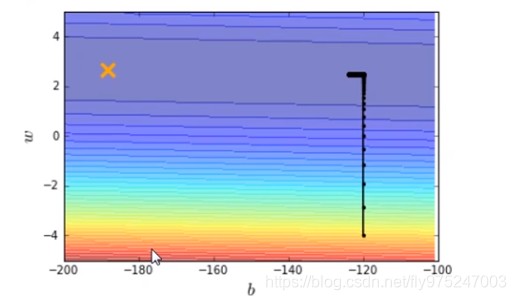
横坐标是b，纵坐标是w，标记×位最优解，显然，在图中我们并没有运行得到最优解，最优解十分的遥远。那么我们就调大learning rate，lr = 0.000001（调大10倍），得到结果如下图。

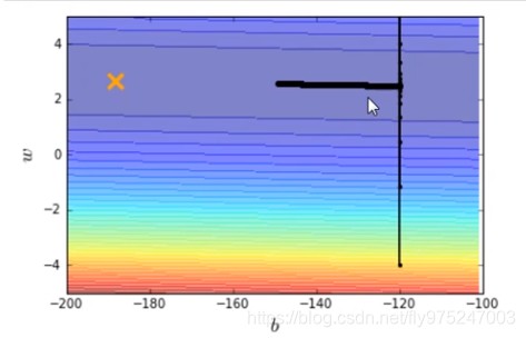
我们再调大learning rate，lr = 0.00001（调大10倍），得到结果如下图。

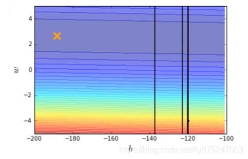
结果发现learning rate太大了，结果很不好。

所以我们给b和w特制化两种learning rate

# linear regression b = -120 w = -4 lr = 1 iteration = 100000 b_history = [b] w_history = [w] lr_b=0 lr_w=0 import time start = time.time() for i in range(iteration): b_grad=0.0 w_grad=0.0 for n in range(len(x_data)) b_grad=b_grad-2.0*(y_data[n]-n-w*x_data[n])*1.0 w_grad= w_grad-2.0*(y_data[n]-n-w*x_data[n])*x_data[n] lr_b=lr_b+b_grad**2 lr_w=lr_w+w_grad**2 # update param b -= lr/np.sqrt(lr_b) * b_grad w -= lr np.sqrt(lr_w) * w_grad b_history.append(b) w_history.append(w)

1234567891011121314151617181920212223242526272829

# plot the figure plt.subplot(1, 2, 1) C = plt.contourf(x, y, Z, 50, alpha=0.5, cmap=plt.get_cmap('jet')) # 填充等高线 # plt.clabel(C, inline=True, fontsize=5) plt.plot([-188.4], [2.67], 'x', ms=12, mew=3, color="orange") plt.plot(b_history, w_history, 'o-', ms=3, lw=1.5, color='black') plt.xlim(-200, -100) plt.ylim(-5, 5) plt.xlabel(r'$b$') plt.ylabel(r'$w$') plt.title("线性回归") plt.subplot(1, 2, 2) loss = np.asarray(loss_history[2:iteration]) plt.plot(np.arange(2, iteration), loss) plt.title("损失") plt.xlabel('step') plt.ylabel('loss') plt.show()

1234567891011121314151617181920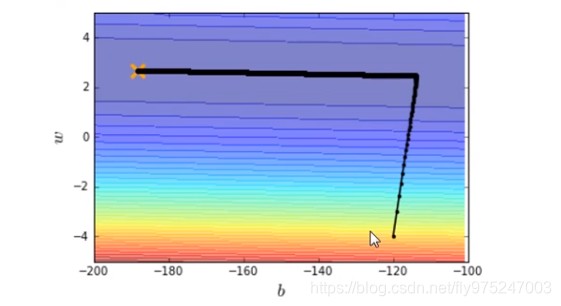

有了新的特制化两种learning rate就可以在10w次迭代之内到达最优点了。

网址：李弘毅机器学习笔记：回归演示 https://www.yuejiaxmz.com/news/view/346800

相关内容

机器学习day01——笔记
机器学习——线性回归基础
李子柒回归爆火！网友：每一帧都是对生活的热爱
最简单的机器学习入门：线性回归
看丹观察丨李子柒回归爆火！网友：每一帧都是对生活的热爱
提高学习效率——5R笔记法
2024黄子弘凡北京演唱会观演攻略（时间+地点+门票）
李毅中：电动车要重视制造和报废、回收再制造阶段的减碳减排
2022学生养成良好的学习习惯演讲稿（精选12篇）
吴恩达深度学习笔记

随便看看